“One Backtest Might Just Be Lucky”, which is the 3rd in my series of short videos with the new Quantifiable Edges Correlation Tool, has been posted to the Quantifiable Edges YouTube channel.
The Correlation Tool can be accessed under Extras -> Correlation Tool for anyone that is logged in to the site. Free access simply requires a login (name & email). Signup here.
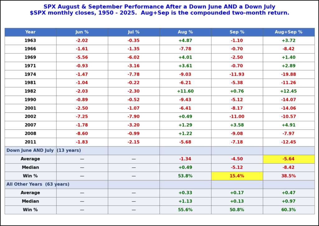
Both June and July saw SPX close lower. Seasonality for those two months it is generally favorable. But since 1950, two of the weakest months are August (3rd worst) and September (worst). So in this weekend’s letter I decided to see how August and September fared when we already had June and July slipping. The table below gives us an answer.
After down closes in both June and July. August has generally been a toss-up. Sometimes it got a bit of a rebound and sometimes it didn’t. But regardless of whether August rebounded or not, September numbers look pretty terrible. Eleven out of the thirteen Septembers closed lower and many of them by sizable amounts. This seems worth keeping in mind while we consider other intermediate-term evidence that emerges over the next 3-4 weeks.
“How Changing Correlation Impacts the Range of Probable Outcomes”, which is the 2nd in my series of short videos with the new Quantifiable Edges Correlation Tool, has been posted to the Quantifiable Edges YouTube channel.
The Correlation Tool can be accessed under Extras -> Correlation Tool for anyone that is logged in to the site. Free access simply requires a login (name & email). Signup here.
“Three Benefits of (Non)Correlation”, which is the 1st in my series of short videos with the new Quantifiable Edges Correlation Tool, has been posted to the Quantifiable Edges YouTube channel.
The Correlation Tool can be accessed under Extras -> Correlation Tool for anyone that is logged in to the site. Free access simply requires a login (name & email). Signup here.
Or how about a free trial to the Quantifiable Edges Gold subscription?
I am excited to introduce the Quantifiable Edges Hypothetical Correlation Tool. I find a lot of people understand diversification, but few grasp how important correlation is when choosing diversifiers. Combining strategies that don’t move in lockstep is a huge key for improving the risk and return of the whole. It’s easy to say “diversification works.” It’s much harder to grasp why, or to see how much. Hopefully our new Hypothetical Correlation Tool will help make that clearer.
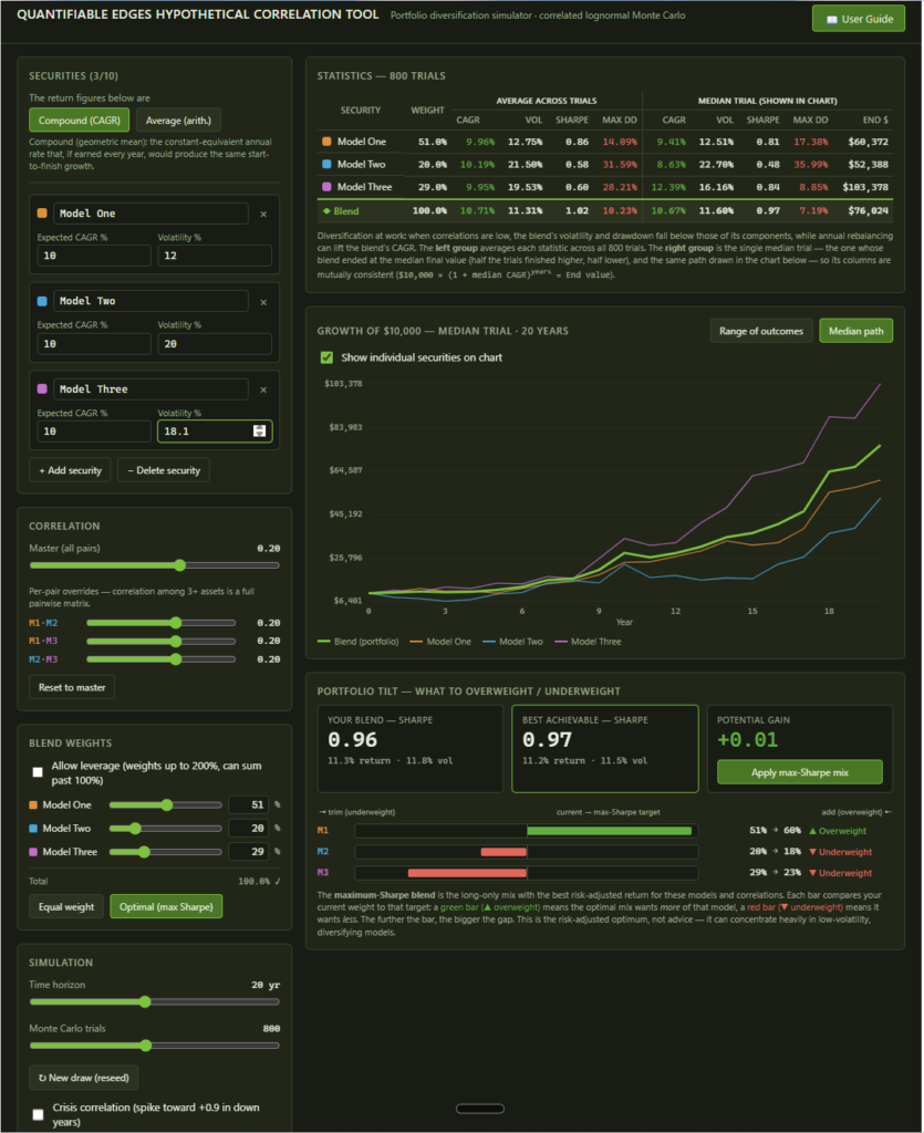
The Hypothetical Correlation Tool lets you define a handful of “models” (each just an expected return and a volatility), choose how correlated they are, decide how much of each to hold, and then watch a Monte Carlo simulation play out thousands of hypothetical futures. It reports the blended portfolio’s compound return, volatility, Sharpe ratio, and worst drawdown, draws the growth of $10,000, and even shows you which models to overweight or underweight to maximize risk-adjusted return. Here is a quick look:
A few things you can explore in about two minutes:
Drag a correlation slider from +1 toward −1 and watch a blend’s volatility melt away while its return holds up.
Flip on “crisis correlation” to see why diversification tends to fail exactly when you need it most.
Hit “new draw” a few times to feel how much any single backtest is just luck.
Check out the “User Guide” (button top right) for more detailed instruction on how to use the tool.
Note: These are not real returns and not a forecast of any strategy. Every number it produces is a hypothetical simulation generated by a mathematical model, for educational purposes only. It’s built only to illustrate the mechanics of diversification and correlation.
I’ll be doing series of posts and short demos where I will use the tool to walk through specific ideas. These include the rebalancing bonus, the limits of diversification in a crash, and the math of leverage. I hope you like the tool. Stay tuned for the first few mini-demos!
To access the tool you simply need to login to Quantifiable Edges. (Even an old expired trial will work.) Once logged in, simply look for the Correlation Tool under the “Extras” menu item. If you don’t have a Quantifiable Edges login, you can sign up for the Correlation Tool (free) here.
Here is a new video I just posted to the Quantifiable Edges YouTube channel showing how I use Claude Code to build models and optimizations in RealTest.
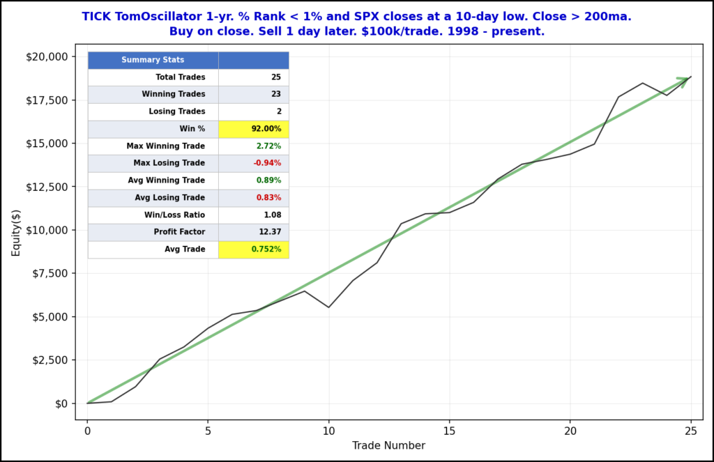
Using closing TICK values as a sentiment indicator is something I learned a long time ago my friend and fellow market analyst, Tom McClellan of McClellan Financial Publications (click for Tom’s article on closing TICK). Tom uses the NYSE closing TICK readings to measure recent end-of-day sentiment. I introduced the TICK Tomoscillator several years ago. For those that are not familiar with the TICK Tomoscillator, you may find a detailed description in the May 13, 2011 blog. The Tomoscillator % Rank Friday came in below 1%, meaning Friday’s reading is among the lowest 1% in the last year. The study below uses the Tomoscillator % Rank reading rather than just the raw reading.
With 23 of 25 instances closing up the next day, there has been a strong bullish inclination. And the line going from lower left to upper right is extremely straight. This is the first time this study has triggered since 2024, but I’ve liked it for a long time and it’s always on my radar.
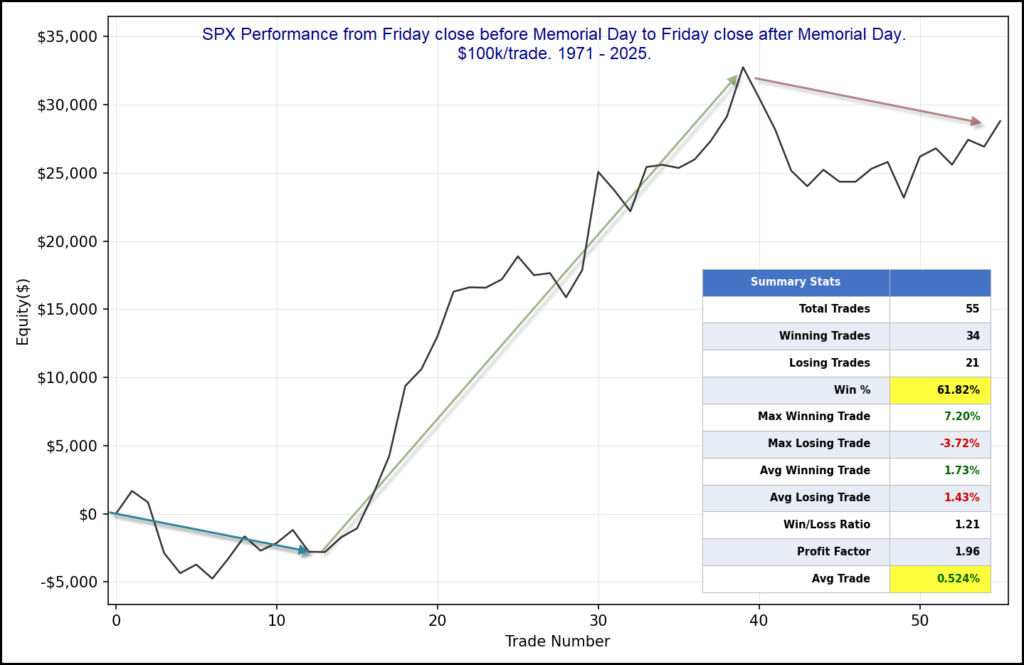
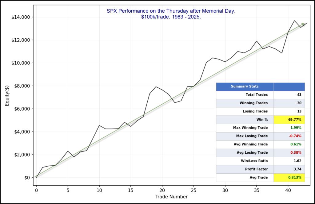
The week of Memorial Day has shown some interesting tendencies over the years. It has been less consistent recently. The chart below examines SPX performance from the Friday before Memorial Day to the Friday after it.
There was no substantial edge apparent throughout the 70s, but starting in 1983 through 2009 there was a substantial bullish tendency. The last 16 years this week has seen more of a struggle. But there remains one day during Memorial Day week where the upside tendency seems to have persisted. That day is Thursday.
A 70% win rate and a strong, steady move higher suggest Thursday looks like a pretty good day from a seasonal standpoint. Traders may want to keep this in mind for later this week.
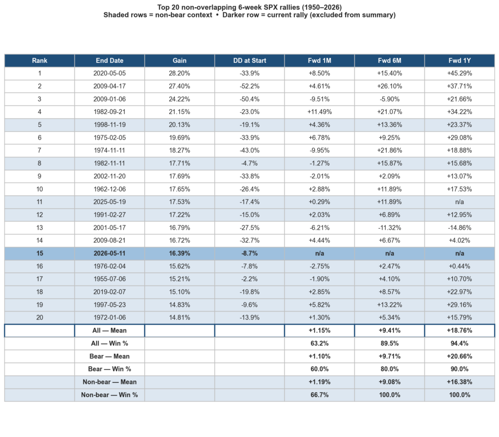
A few days ago on X, Charlie Bilello pointed out SPX had gained more than 16% over the previous six weeks and that’s one of the biggest six-week rallies of all time. I looked back at the top 20 non-overlapping 30-trading-day rallies since 1950. They can all be found in the table below.
Shaded rows are those instances where there was less than a 20% drawdown at the start of the rally. The current instance saw one of the shallower drawdowns. Only 1955, 1976, and 1982 saw rallies that were not coming out of larger drawdowns than the current one. After such strong rallies whether they were bear or non-bear, the next month generally did not see much progress. But longer-term results were quite impressive. After the 19 prior 6-week rallies, SPX averaged +18.8% over the next year with a 94.4% win rate, versus a +9.4% / 74.5% baseline. Below you can see the signal versus the baseline numbers.
Signal vs baseline forward returns (top 20 rallies)
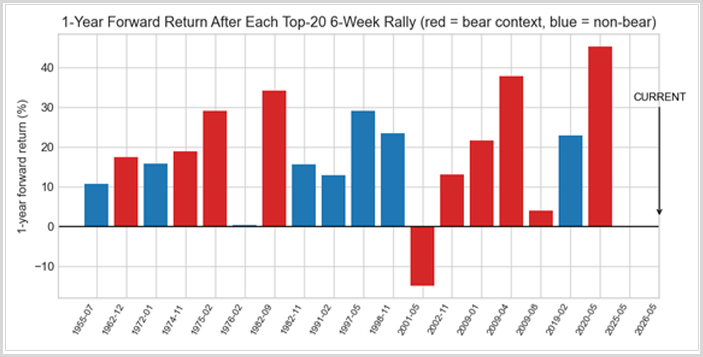
Lastly a little graphic showing the one-year forward returns after each of the 6-week rallies:
So the momentum over the recent six-week period seems to be positive. We’ve seen this other ways but I thought this was an interesting look. Also impressive is that looking at the eight non-bear instances the average drawdown was only 8.29%, while the average run-up was 18.96%. There are certainly risks out there, but strong moves like we have seen recently tend to be a positive over the intermediate and long term.
For much of last week I was at the National Association of Active Investment Managers (NAAIM) Uncommon Knowledge conference. NAAIM is a terrific organization that I have become more involved with over the years.
NAAIM has published its “NAAIM Exposure Index” since 2006. I did some research a few years ago on the index to determine whether the numbers might be valuable as part of a model. I found that 1) strongly oversold readings could be indicative that the market is so oversold it is ready to rally, 2) strongly overbought readings are not a contrarian indicator. In fact they often suggest strong momentum that is likely to continue. I had a discussion with some NAAIM members a few weeks back. The topic was the Exposure Index: who used it, what they used it for, and where was the actual value in it?
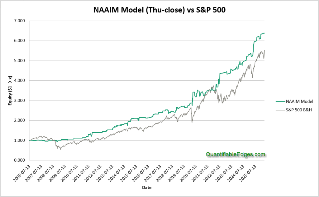
So I decided to revisit my old research and see if I could create a model based on those concepts that could demonstrate the value that the index provides. Results came out better than anticipated. Below is a look at the profit curve of the model versus the S&P 500.
The NAAIM Exposure Index is released each week during market hours on Thursday. So the model trades at the close every Thursday afternoon. (Thanksgiving and other holidays will sometimes bump it forward one day.) There are three setups that will cause the model to go long.
This week’s reading is among the bottom 10% of readings seen over the last 52 weeks (one year). Additionally, it is not lower than last week’s reading. Essentially this is looking for a strongly oversold reading, but not looking to catch a falling knife. So we want to see the Exposure Index near or slightly above where it was the week before.
This week’s reading is at least 80 and it has risen at least 15 points over the last four weeks. This is looking for strong and growing enthusiasm.
This week’s reading is at least 100. As it turns out, when you have a bunch of smart investment managers getting leveraged, there is a good chance that they are right and that there are market gains ahead.
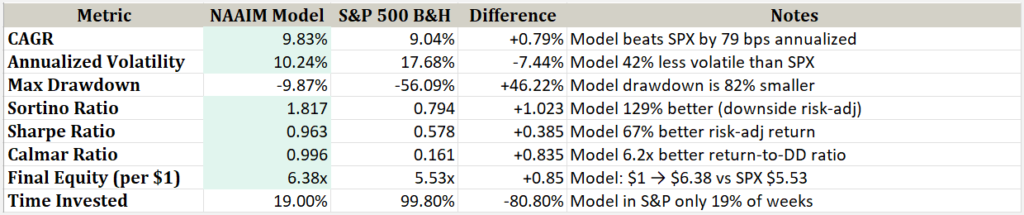
If any one of the above is true, the model will go (or remain) long 150% SPX at the close on Thursday, and will remain long at least until the following Thursday when the new number is published. Below is a stats table summarizing the results.
The numbers here compare very favorably to the SPX. Leverage when there is an edge and cash when there is not. As you can see the model’s only invested 19% of the time. That is a big risk reducer. One thing to note is the Max Drawdown. It is shown as less than 10% in the table above. But that is partially because this model is just using weekly closing numbers. I created a version in Realtest that uses daily pricing. And thanks to March 2020, the max drawdown reached 25% using daily bars. (Still less than half that of the S&P 500.)
Is this a model I would actually trade? No. I don’t think I’d trade any model where I had to hold for a full week based solely on survey results. Of course the fact that it is built solely on survey results, and does not take into account price, or trend, or volume, or breadth, or anything else, is what really demonstrates the value of the NAAIM Exposure Index. And that was kind of the whole point. Trading solely on the index may be overenthusiastic but utilizing it as one input within a larger model seems completely reasonable and could very possibly strengthen it.
I have the model available in both Excel and Realtest format. If you have a username and password at Quantifiable Edges, then you can download the model from the Other Code and Spreadsheets page. If you don’t have a log-in, you can get one by simply signing up for a free trial! And if you don’t want a free trial right now, then just join our email list and you will receive a copy. Easy as pie.
Disclaimer: The performance shown above is hypothetical and does not represent an actual trading account. Results were generated frictionlessly, meaning they do not include commissions, slippage, or other costs that would be incurred in live trading. Past performance, actual or hypothetical, is no guarantee of future results.
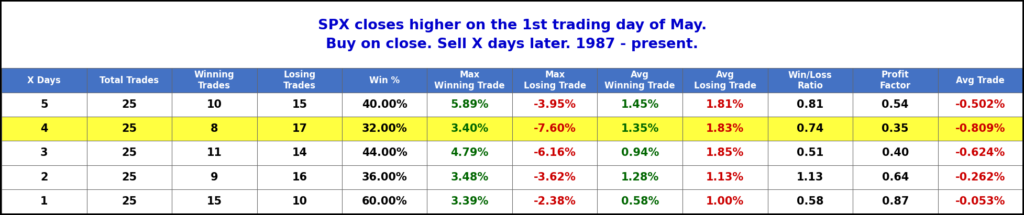
May got off to a positive start. But a strong start to May has typically been followed by a dip in the next few days. This can be seen in the study below, which was featured in this weekend’s subscriber letter.
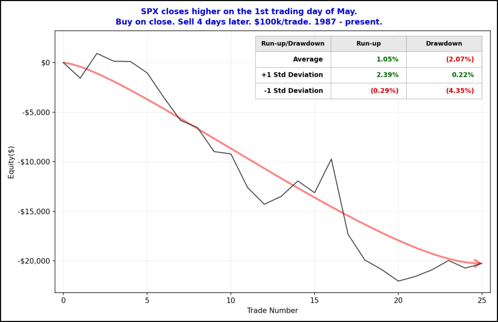
Of the 25 instances that rose on the first day in May since 1987, 17 of them closed lower 4 days later. Below is an equity curve that shows how it has played out over time.
I’ll note the big drop in instance 17 was the 2010 Flash Crash. Even without that instance there appears to be a solid downside inclination.
I will also note that while seasonality appears negative over the next few days, there was quite a mix of bullish and bearish studies featured in the subscriber letter over the weekend. I don’t view this as a reason to trade on its own, but it is a tendency that traders may want to consider.
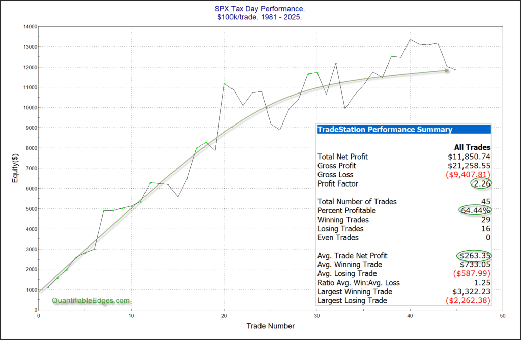
April 15th is tax day. Tax day has historically been a good day for the market. A reason tax day may be bullish is that it is the last day that people can make IRA contributions to count for the previous tax year. This can create a last-minute rush and you will often have an inflow of funds heading into the market right around and on April 15th (or whenever tax day ends up falling, since it is sometimes delayed). Fund managers will often put this money to work immediately and it creates a positive bias for the market. But the edge has not played out as well in recent years. This can be seen in the chart below.
Is it still potentially bullish? I believe so. Is it the layup that it once appeared to be? No. But I still find it interesting and perhaps worth consideration when thinking about Wednesday’s potential.
Note: Later this week I will be having the annual “Black Friday” sale, which is the only sale I run during the year. If you think you might be interested in a subscription, then now might be a good time to take a free 1-week trial and see if Quantifiable Edges would be helpful for you…
The time around Thanksgiving has shown some strong tendencies – both bullish and bearish. I have discussed them a number of times over the years. In the updated table below I show SPX performance results based on the day of the week around Thanksgiving. The bottom row is the Monday after Thanksgiving week. The top row is the Monday before Thanksgiving.
Monday and Tuesday of Thanksgiving week do not show a strong, consistent edge. But the data for both Wednesday and Friday looks quite strong. Wednesday has had the most consistent gains (76.9%), and the largest average p/l of 0.3% ($297.44 on $100k.) Friday’s stats look fairly impressive, but it has not performed nearly as well over the last 15 years as it had previously. Meanwhile, the Monday after Thanksgiving has given back a good chunk of the gains that were realized on Wednesday and Friday. The worst “Monday After” came in 2008 with a 9% 1-day decline. Since then, Monday After performance has been basically breakeven.
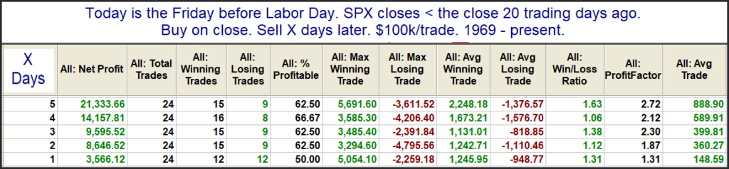
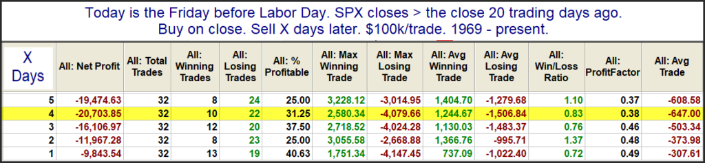
In the subscriber letter over the last several years I have demonstrated that the performance during the week of Labor Day has been impacted by the performance in the month leading up to it. Interestingly, is has been somewhat of a momentum reversal week. When SPX has rallied up to Labor Day, then it has struggled that week. And declines into Labor Day have seen positive performance. Below is an updated look at the two scenarios.
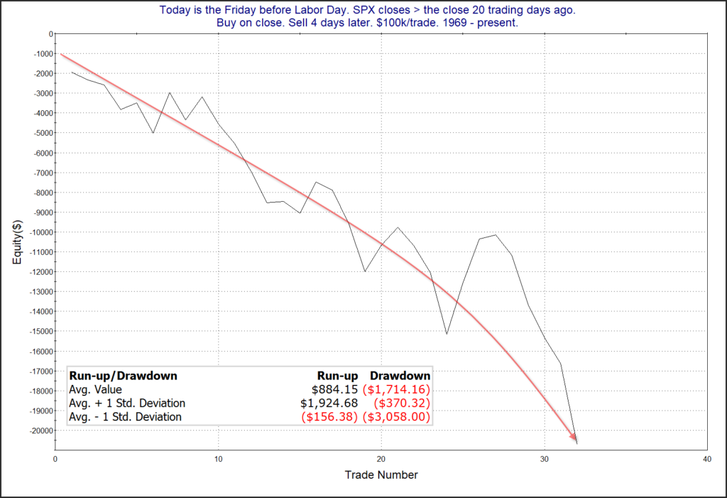
The 4-day numbers are basically inverted. So the Tues-Fri after Labor Day have not seen any consistency without the delineator. But the trend filter reveals a striking difference. Over the last several weeks the market has rallied nicely, so we are currently facing the 2nd scenario. Below is a look at the profit curve for the 4-day exit following the current setup.
Choppy but an obvious downslope. Traders may want to consider this for the upcoming trading week. Have a great Labor Day!
To see other studies featured in this weekend’s subscriber letter, check out a free trial.
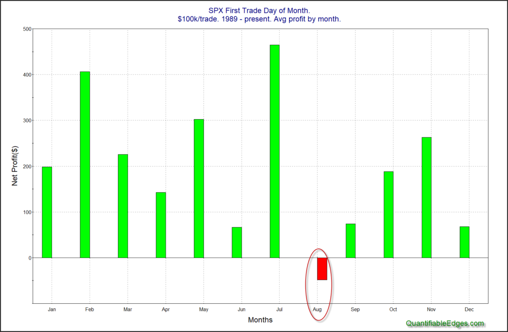
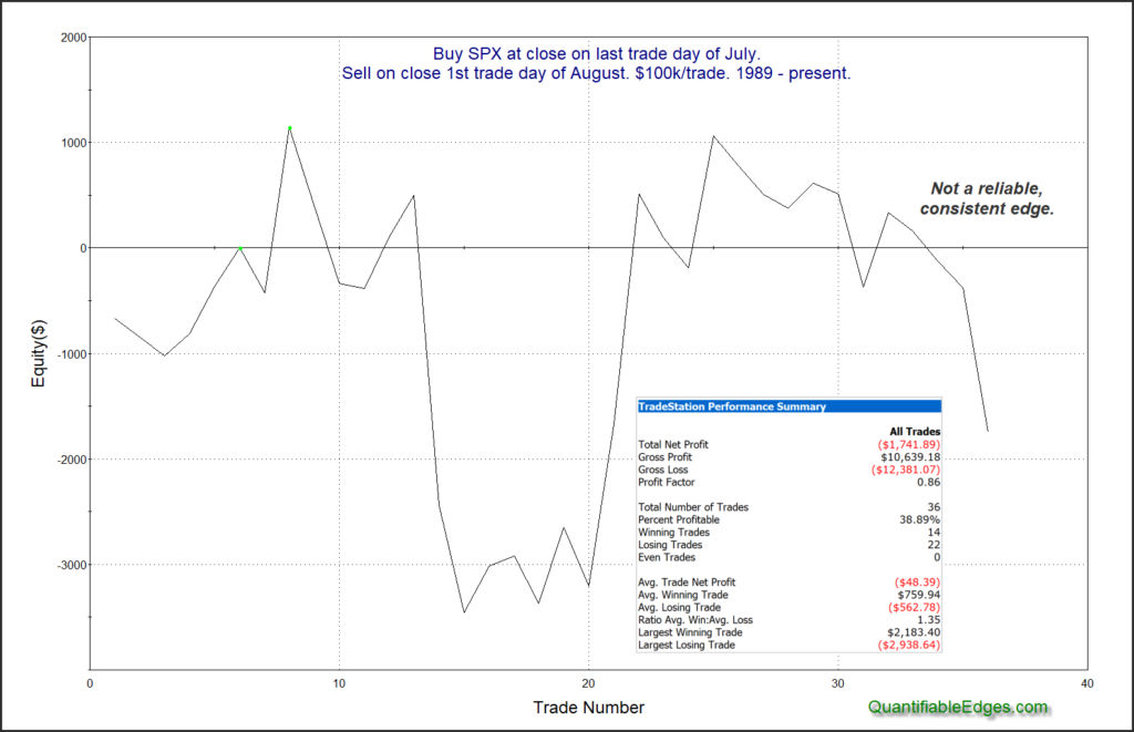
I’ve shown the chart below several times over the years. It breaks down by month the performance of the first trading day of the month. July has long had the strongest Day 1. But August is also notable for it’s lack of Day 1 performance.
As you can see it is the only month with a negative Day 1 return. Below is a look at how it has played out over time.
This doesn’t appear to be a bearish setup. Just a bunch of chop that has failed to generate gains over time. But while it doesn’t hint at a down day on August 1st, it certainly shows that August 1 has certainly not been seasonally bullish.